I am happy to introduce the rbin package, a set of tools for binning/discretization of data, designed keeping in mind beginner/intermediate R users. It includes two RStudio addins for interactive binning.
Installation
# Install release version from CRAN
install.packages("rbin")

# Install development version from GitHub
# install.packages("devtools")
devtools::install_github("rsquaredacademy/rbin")
RStudio Addins
rbin includes two RStudio addins for manually binning data. Below is a demo:
Read on to learn more about the features of rbin, or see the rbin website for detailed documentation on using the package.
Introduction
Binning is the process of transforming numerical or continuous data into categorical data. It is a common data pre-processing step of the model building process. rbin has the following features:
- manual binning using shiny app
- equal length binning method
- winsorized binning method
- quantile binning method
- combine levels of categorical data
- create dummy variables based on binning method
- calculates weight of evidence (WOE), entropy and information value (IV)
- provides summary information about binning process
Manual Binning
For manual binning, you need to specify the cut points for the bins. rbin
follows the left closed and right open interval ([0,1) = {x | 0 ≤ x < 1}) for
creating bins. The number of cut points you specify is one less than the number
of bins you want to create i.e. if you want to create 10 bins, you need to
specify only 9 cut points as shown in the below example. The accompanying
RStudio addin, rbinAddin() can be used to iteratively bin the data and to
enforce monotonic increasing/decreasing trend.
After finalizing the bins, you can use rbin_create() to create the dummy
variables.
Bins
bins <- rbin_manual(mbank, y, age, c(29, 31, 34, 36, 39, 42, 46, 51, 56))
bins
## Binning Summary
## ---------------------------
## Method Manual
## Response y
## Predictor age
## Bins 10
## Count 4521
## Goods 517
## Bads 4004
## Entropy 0.5
## Information Value 0.12
##
##
## # A tibble: 10 x 7
## cut_point bin_count good bad woe iv entropy
## <chr> <int> <int> <int> <dbl> <dbl> <dbl>
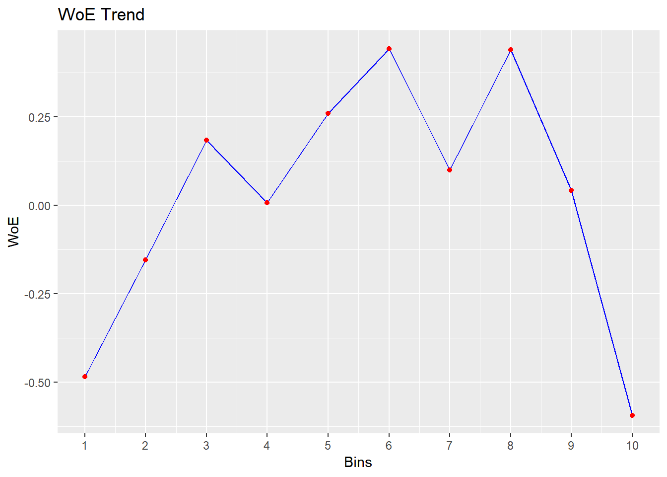
## 1 < 29 410 71 339 -0.484 0.0255 0.665
## 2 < 31 313 41 272 -0.155 0.00176 0.560
## 3 < 34 567 55 512 0.184 0.00395 0.459
## 4 < 36 396 45 351 0.00712 0.00000443 0.511
## 5 < 39 519 47 472 0.260 0.00701 0.438
## 6 < 42 431 33 398 0.443 0.0158 0.390
## 7 < 46 449 47 402 0.0993 0.000942 0.484
## 8 < 51 521 40 481 0.440 0.0188 0.391
## 9 < 56 445 49 396 0.0426 0.000176 0.500
## 10 >= 56 470 89 381 -0.593 0.0456 0.700Plot
plot(bins)
Dummy Variables
bins <- rbin_manual(mbank, y, age, c(29, 31, 34, 36, 39, 42, 46, 51, 56))
rbin_create(mbank, age, bins)
## # A tibble: 4,521 x 26
## age job marital education default balance housing loan
## <int> <fct> <fct> <fct> <fct> <dbl> <fct> <fct>
## 1 34 technician married tertiary no 297 yes no
## 2 49 services married secondary no 180 yes yes
## 3 38 admin. single secondary no 262 no no
## 4 47 services married secondary no 367 yes no
## 5 51 self-employed single secondary no 1640 yes no
## 6 40 unemployed married secondary no 3382 yes no
## 7 58 retired married secondary no 1227 no no
## 8 32 unemployed married primary no 309 yes no
## 9 46 blue-collar married secondary no 922 yes no
## 10 32 services married tertiary no 0 no no
## contact day month duration campaign pdays previous poutcome y
## <fct> <int> <fct> <int> <int> <int> <int> <fct> <fct>
## 1 cellular 29 jan 375 2 -1 0 unknown 0
## 2 unknown 2 jun 392 3 -1 0 unknown 0
## 3 cellular 3 feb 315 2 180 6 failure 1
## 4 cellular 12 may 309 1 306 4 success 1
## 5 unknown 15 may 67 4 -1 0 unknown 0
## 6 unknown 14 may 125 1 -1 0 unknown 0
## 7 cellular 14 aug 182 2 37 2 failure 0
## 8 telephone 13 may 185 1 370 3 failure 0
## 9 telephone 18 nov 296 2 -1 0 unknown 0
## 10 cellular 21 nov 80 1 -1 0 unknown 0
## `age_<_31` `age_<_34` `age_<_36` `age_<_39` `age_<_42` `age_<_46`
## <dbl> <dbl> <dbl> <dbl> <dbl> <dbl>
## 1 0 0 1 0 0 0
## 2 0 0 0 0 0 0
## 3 0 0 0 1 0 0
## 4 0 0 0 0 0 0
## 5 0 0 0 0 0 0
## 6 0 0 0 0 1 0
## 7 0 0 0 0 0 0
## 8 0 1 0 0 0 0
## 9 0 0 0 0 0 0
## 10 0 1 0 0 0 0
## `age_<_51` `age_<_56` `age_>=_56`
## <dbl> <dbl> <dbl>
## 1 0 0 0
## 2 1 0 0
## 3 0 0 0
## 4 1 0 0
## 5 0 1 0
## 6 0 0 0
## 7 0 0 1
## 8 0 0 0
## 9 1 0 0
## 10 0 0 0
## # ... with 4,511 more rowsFactor Binning
You can collapse or combine levels of a factor/categorical variable using
rbin_factor_combine() and then use rbin_factor() to look at weight of
evidence, entropy and information value. After finalizing the bins, you can
use rbin_factor_create() to create the dummy variables. You can use the
RStudio addin, rbinFactorAddin() to interactively combine the levels and
create dummy variables after finalizing the bins.
Combine Levels
upper <- c("secondary", "tertiary")
out <- rbin_factor_combine(mbank, education, upper, "upper")
table(out$education)
##
## primary unknown upper
## 691 179 3651out <- rbin_factor_combine(mbank, education, c("secondary", "tertiary"), "upper")
table(out$education)##
## primary unknown upper
## 691 179 3651Bins
bins <- rbin_factor(mbank, y, education)
bins
## Binning Summary
## ---------------------------
## Method Custom
## Response y
## Predictor education
## Levels 4
## Count 4521
## Goods 517
## Bads 4004
## Entropy 0.51
## Information Value 0.05
##
##
## # A tibble: 4 x 7
## level bin_count good bad woe iv entropy
## <fct> <int> <int> <int> <dbl> <dbl> <dbl>
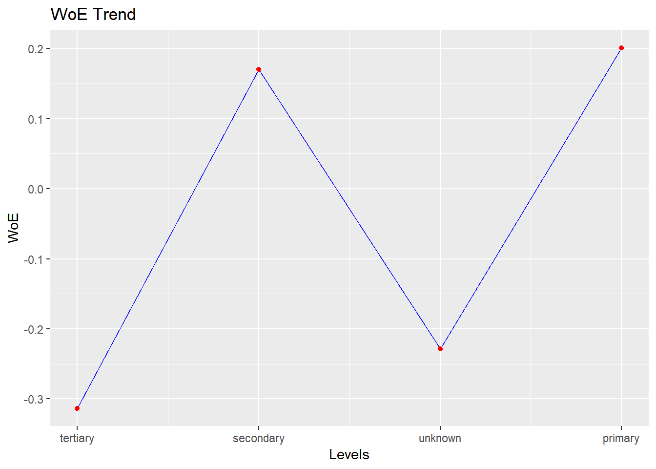
## 1 tertiary 1299 195 1104 -0.313 0.0318 0.610
## 2 secondary 2352 231 2121 0.170 0.0141 0.463
## 3 unknown 179 25 154 -0.229 0.00227 0.583
## 4 primary 691 66 625 0.201 0.00572 0.455Plot
plot(bins)
Create Bins
upper <- c("secondary", "tertiary")
out <- rbin_factor_combine(mbank, education, upper, "upper")
rbin_factor_create(out, education)
## # A tibble: 4,521 x 19
## age job marital default balance housing loan contact
## <int> <fct> <fct> <fct> <dbl> <fct> <fct> <fct>
## 1 34 technician married no 297 yes no cellular
## 2 49 services married no 180 yes yes unknown
## 3 38 admin. single no 262 no no cellular
## 4 47 services married no 367 yes no cellular
## 5 51 self-employed single no 1640 yes no unknown
## 6 40 unemployed married no 3382 yes no unknown
## 7 58 retired married no 1227 no no cellular
## 8 32 unemployed married no 309 yes no telephone
## 9 46 blue-collar married no 922 yes no telephone
## 10 32 services married no 0 no no cellular
## day month duration campaign pdays previous poutcome y education
## <int> <fct> <int> <int> <int> <int> <fct> <fct> <fct>
## 1 29 jan 375 2 -1 0 unknown 0 upper
## 2 2 jun 392 3 -1 0 unknown 0 upper
## 3 3 feb 315 2 180 6 failure 1 upper
## 4 12 may 309 1 306 4 success 1 upper
## 5 15 may 67 4 -1 0 unknown 0 upper
## 6 14 may 125 1 -1 0 unknown 0 upper
## 7 14 aug 182 2 37 2 failure 0 upper
## 8 13 may 185 1 370 3 failure 0 primary
## 9 18 nov 296 2 -1 0 unknown 0 upper
## 10 21 nov 80 1 -1 0 unknown 0 upper
## education_unknown education_upper
## <dbl> <dbl>
## 1 0 1
## 2 0 1
## 3 0 1
## 4 0 1
## 5 0 1
## 6 0 1
## 7 0 1
## 8 0 0
## 9 0 1
## 10 0 1
## # ... with 4,511 more rowsQuantile Binning
Quantile binning aims to bin the data into roughly equal groups using quantiles.
bins <- rbin_quantiles(mbank, y, age, 10)
bins
## Binning Summary
## -----------------------------
## Method Quantile
## Response y
## Predictor age
## Bins 10
## Count 4521
## Goods 517
## Bads 4004
## Entropy 0.5
## Information Value 0.12
##
##
## # A tibble: 10 x 7
## cut_point bin_count good bad woe iv entropy
## <chr> <int> <int> <int> <dbl> <dbl> <dbl>
## 1 < 29 410 71 339 -0.484 0.0255 0.665
## 2 < 31 313 41 272 -0.155 0.00176 0.560
## 3 < 34 567 55 512 0.184 0.00395 0.459
## 4 < 36 396 45 351 0.00712 0.00000443 0.511
## 5 < 39 519 47 472 0.260 0.00701 0.438
## 6 < 42 431 33 398 0.443 0.0158 0.390
## 7 < 46 449 47 402 0.0993 0.000942 0.484
## 8 < 51 521 40 481 0.440 0.0188 0.391
## 9 < 56 445 49 396 0.0426 0.000176 0.500
## 10 >= 56 470 89 381 -0.593 0.0456 0.700Plot
plot(bins)
Winsorized Binning
Winsorized binning is similar to equal length binning except that both tails are cut off to obtain a smooth binning result. This technique is often used to remove outliers during the data pre-processing stage. For Winsorized binning, the Winsorized statistics are computed first. After the minimum and maximum have been found, the split points are calculated the same way as in equal length binning.
bins <- rbin_winsorize(mbank, y, age, 10, winsor_rate = 0.05)
bins
## Binning Summary
## ------------------------------
## Method Winsorize
## Response y
## Predictor age
## Bins 10
## Count 4521
## Goods 517
## Bads 4004
## Entropy 0.51
## Information Value 0.1
##
##
## # A tibble: 10 x 7
## cut_point bin_count good bad woe iv entropy
## <chr> <int> <int> <int> <dbl> <dbl> <dbl>
## 1 < 30.2 723 112 611 -0.350 0.0224 0.622
## 2 < 33.4 567 55 512 0.184 0.00395 0.459
## 3 < 36.6 573 58 515 0.137 0.00225 0.473
## 4 < 39.8 497 44 453 0.285 0.00798 0.432
## 5 < 43 396 37 359 0.225 0.00408 0.448
## 6 < 46.2 461 43 418 0.227 0.00482 0.447
## 7 < 49.4 281 22 259 0.419 0.00927 0.396
## 8 < 52.6 309 32 277 0.111 0.000811 0.480
## 9 < 55.8 244 25 219 0.123 0.000781 0.477
## 10 >= 55.8 470 89 381 -0.593 0.0456 0.700Plot
plot(bins)
Learning More
The rbin website includes comprehensive documentation on using the package, including the following article that gives a brief introduction to rbin:
Feedback
rbin has been on CRAN for a few months now while we were fixing bugs and making the API stable. All feedback is welcome. Issues (bugs and feature requests) can be posted to github tracker. For help with code or other related questions, feel free to reach out to us at pkgs@rsquaredacademy.com.