# Install release version from CRAN
install.packages("descriptr")

# Install development version from GitHub
# install.packages("devtools")
devtools::install_github("rsquaredacademy/descriptr")Descriptive Statistics in R
summary statistics
Tools for descriptive statistics in R.
I am pleased to announce the descriptr package, a set of tools for generating descriptive/summary statistics.
Installation
Shiny App
descriptr includes a shiny app which can be launched using
ds_launch_shiny_app()or try the live version here.
Read on to learn more about the features of descriptr, or see the descriptr website for detailed documentation on using the package.
Warning: package 'descriptr' was built under R version 4.5.3Warning: package 'dplyr' was built under R version 4.5.3Data
We have modified the mtcars data to create a new data set mtcarz. The only difference between the two data sets is related to the variable types.
str(mtcarz)'data.frame': 32 obs. of 11 variables:
$ mpg : num 21 21 22.8 21.4 18.7 18.1 14.3 24.4 22.8 19.2 ...
$ cyl : Factor w/ 3 levels "4","6","8": 2 2 1 2 3 2 3 1 1 2 ...
$ disp: num 160 160 108 258 360 ...
$ hp : num 110 110 93 110 175 105 245 62 95 123 ...
$ drat: num 3.9 3.9 3.85 3.08 3.15 2.76 3.21 3.69 3.92 3.92 ...
$ wt : num 2.62 2.88 2.32 3.21 3.44 ...
$ qsec: num 16.5 17 18.6 19.4 17 ...
$ vs : Factor w/ 2 levels "0","1": 1 1 2 2 1 2 1 2 2 2 ...
$ am : Factor w/ 2 levels "0","1": 2 2 2 1 1 1 1 1 1 1 ...
$ gear: Factor w/ 3 levels "3","4","5": 2 2 2 1 1 1 1 2 2 2 ...
$ carb: Factor w/ 6 levels "1","2","3","4",..: 4 4 1 1 2 1 4 2 2 4 ...Data Screening
The ds_screener() function will screen a data set and return the following: - Column/Variable Names - Data Type - Levels (in case of categorical data) - Number of missing observations - % of missing observations
ds_screener(mtcarz)-----------------------------------------------------------------------
| Column Name | Data Type | Levels | Missing | Missing (%) |
-----------------------------------------------------------------------
| mpg | numeric | NA | 0 | 0 |
| cyl | factor | 4 6 8 | 0 | 0 |
| disp | numeric | NA | 0 | 0 |
| hp | numeric | NA | 0 | 0 |
| drat | numeric | NA | 0 | 0 |
| wt | numeric | NA | 0 | 0 |
| qsec | numeric | NA | 0 | 0 |
| vs | factor | 0 1 | 0 | 0 |
| am | factor | 0 1 | 0 | 0 |
| gear | factor | 3 4 5 | 0 | 0 |
| carb | factor |1 2 3 4 6 8| 0 | 0 |
-----------------------------------------------------------------------
Overall Missing Values 0
Percentage of Missing Values 0 %
Rows with Missing Values 0
Columns With Missing Values 0 Continuous Data
Summary Statistics
The ds_summary_stats function returns a comprehensive set of statistics including measures of location, variation, symmetry and extreme observations.
ds_summary_stats(mtcarz, mpg)-------------------------------- Variable: mpg --------------------------------
Univariate Analysis
N 32.00 Variance 36.32
Missing 0.00 Std Deviation 6.03
Mean 20.09 Range 23.50
Median 19.20 Interquartile Range 7.38
Mode 10.40 Uncorrected SS 14042.31
Trimmed Mean 19.95 Corrected SS 1126.05
Skewness 0.67 Coeff Variation 30.00
Kurtosis -0.02 Std Error Mean 1.07
Quantiles
Quantile Value
Max 33.90
99% 33.44
95% 31.30
90% 30.09
Q3 22.80
Median 19.20
Q1 15.43
10% 14.34
5% 12.00
1% 10.40
Min 10.40
Extreme Values
Low High
Obs Value Obs Value
15 10.4 20 33.9
16 10.4 18 32.4
24 13.3 19 30.4
7 14.3 28 30.4
17 14.7 26 27.3 You can pass multiple variables as shown below:
ds_summary_stats(mtcarz, mpg, disp)-------------------------------- Variable: mpg --------------------------------
Univariate Analysis
N 32.00 Variance 36.32
Missing 0.00 Std Deviation 6.03
Mean 20.09 Range 23.50
Median 19.20 Interquartile Range 7.38
Mode 10.40 Uncorrected SS 14042.31
Trimmed Mean 19.95 Corrected SS 1126.05
Skewness 0.67 Coeff Variation 30.00
Kurtosis -0.02 Std Error Mean 1.07
Quantiles
Quantile Value
Max 33.90
99% 33.44
95% 31.30
90% 30.09
Q3 22.80
Median 19.20
Q1 15.43
10% 14.34
5% 12.00
1% 10.40
Min 10.40
Extreme Values
Low High
Obs Value Obs Value
15 10.4 20 33.9
16 10.4 18 32.4
24 13.3 19 30.4
7 14.3 28 30.4
17 14.7 26 27.3
-------------------------------- Variable: disp --------------------------------
Univariate Analysis
N 32.00 Variance 15360.80
Missing 0.00 Std Deviation 123.94
Mean 230.72 Range 400.90
Median 196.30 Interquartile Range 205.18
Mode 275.80 Uncorrected SS 2179627.47
Trimmed Mean 228.00 Corrected SS 476184.79
Skewness 0.42 Coeff Variation 53.72
Kurtosis -1.07 Std Error Mean 21.91
Quantiles
Quantile Value
Max 472.00
99% 468.28
95% 449.00
90% 396.00
Q3 326.00
Median 196.30
Q1 120.83
10% 80.61
5% 77.35
1% 72.53
Min 71.10
Extreme Values
Low High
Obs Value Obs Value
20 71.1 15 472
19 75.7 16 460
18 78.7 17 440
26 79 25 400
28 95.1 5 360 If you do not specify any variables, it will detect all the continuous variables in the data set and return summary statistics for each of them.
Frequency Distribution
The ds_freq_table function creates frequency tables for continuous variables. The default number of intervals is 5.
ds_freq_table(mtcarz, mpg, 4) Variable: mpg
|---------------------------------------------------------------------------|
| Bins | Frequency | Cum Frequency | Percent | Cum Percent |
|---------------------------------------------------------------------------|
| 10.4 - 16.3 | 10 | 10 | 31.25 | 31.25 |
|---------------------------------------------------------------------------|
| 16.3 - 22.1 | 13 | 23 | 40.62 | 71.88 |
|---------------------------------------------------------------------------|
| 22.1 - 28 | 5 | 28 | 15.62 | 87.5 |
|---------------------------------------------------------------------------|
| 28 - 33.9 | 4 | 32 | 12.5 | 100 |
|---------------------------------------------------------------------------|
| Total | 32 | - | 100.00 | - |
|---------------------------------------------------------------------------|Histogram
A plot() method has been defined which will generate a histogram.
k <- ds_freq_table(mtcarz, mpg, 4)
plot(k)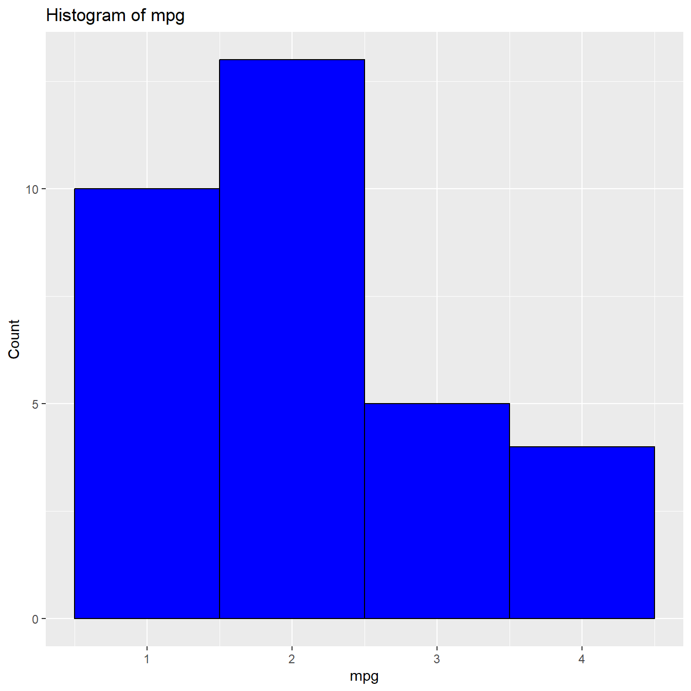
Auto Summary
If you want to view summary statistics and frequency tables of all or subset of variables in a data set, use ds_auto_summary().
ds_auto_summary_stats(mtcarz, disp, mpg)-------------------------------- Variable: disp --------------------------------
------------------------------ Summary Statistics ------------------------------
-------------------------------- Variable: disp --------------------------------
Univariate Analysis
N 32.00 Variance 15360.80
Missing 0.00 Std Deviation 123.94
Mean 230.72 Range 400.90
Median 196.30 Interquartile Range 205.18
Mode 275.80 Uncorrected SS 2179627.47
Trimmed Mean 228.00 Corrected SS 476184.79
Skewness 0.42 Coeff Variation 53.72
Kurtosis -1.07 Std Error Mean 21.91
Quantiles
Quantile Value
Max 472.00
99% 468.28
95% 449.00
90% 396.00
Q3 326.00
Median 196.30
Q1 120.83
10% 80.61
5% 77.35
1% 72.53
Min 71.10
Extreme Values
Low High
Obs Value Obs Value
20 71.1 15 472
19 75.7 16 460
18 78.7 17 440
26 79 25 400
28 95.1 5 360
NULL
---------------------------- Frequency Distribution ----------------------------
Variable: disp
|---------------------------------------------------------------------------|
| Bins | Frequency | Cum Frequency | Percent | Cum Percent |
|---------------------------------------------------------------------------|
| 71.1 - 151.3 | 12 | 12 | 37.5 | 37.5 |
|---------------------------------------------------------------------------|
| 151.3 - 231.5 | 5 | 17 | 15.62 | 53.12 |
|---------------------------------------------------------------------------|
| 231.5 - 311.6 | 6 | 23 | 18.75 | 71.88 |
|---------------------------------------------------------------------------|
| 311.6 - 391.8 | 5 | 28 | 15.62 | 87.5 |
|---------------------------------------------------------------------------|
| 391.8 - 472 | 4 | 32 | 12.5 | 100 |
|---------------------------------------------------------------------------|
| Total | 32 | - | 100.00 | - |
|---------------------------------------------------------------------------|
-------------------------------- Variable: mpg --------------------------------
------------------------------ Summary Statistics ------------------------------
-------------------------------- Variable: mpg --------------------------------

                        Univariate Analysis

 N                       32.00      Variance                36.32
 Missing                  0.00      Std Deviation            6.03
 Mean                    20.09      Range                   23.50
 Median                  19.20      Interquartile Range      7.38
 Mode                    10.40      Uncorrected SS       14042.31
 Trimmed Mean            19.95      Corrected SS          1126.05
 Skewness                 0.67      Coeff Variation         30.00
 Kurtosis                -0.02      Std Error Mean           1.07

                              Quantiles

              Quantile                            Value

             Max                                  33.90
             99%                                  33.44
             95%                                  31.30
             90%                                  30.09
             Q3                                   22.80
             Median                               19.20
             Q1                                   15.43
             10%                                  14.34
             5%                                   12.00
             1%                                   10.40
             Min                                  10.40

                            Extreme Values

                Low                                High

  Obs                        Value       Obs                        Value
  15                         10.4        20                         33.9
  16                         10.4        18                         32.4
  24                         13.3        19                         30.4
   7                         14.3        28                         30.4
  17                         14.7        26                         27.3
NULL
---------------------------- Frequency Distribution ----------------------------
Variable: mpg
|-----------------------------------------------------------------------|
| Bins | Frequency | Cum Frequency | Percent | Cum Percent |
|-----------------------------------------------------------------------|
| 10.4 - 15.1 | 6 | 6 | 18.75 | 18.75 |
|-----------------------------------------------------------------------|
| 15.1 - 19.8 | 12 | 18 | 37.5 | 56.25 |
|-----------------------------------------------------------------------|
| 19.8 - 24.5 | 8 | 26 | 25 | 81.25 |
|-----------------------------------------------------------------------|
| 24.5 - 29.2 | 2 | 28 | 6.25 | 87.5 |
|-----------------------------------------------------------------------|
| 29.2 - 33.9 | 4 | 32 | 12.5 | 100 |
|-----------------------------------------------------------------------|
| Total | 32 | - | 100.00 | - |
|-----------------------------------------------------------------------|Group Summary
The ds_group_summary() function returns descriptive statistics of a continuous variable for the different levels of a categorical variable.
k <- ds_group_summary(mtcarz, cyl, mpg)
k
by
-----------------------------------------------------------------------------------------
| Statistic/Levels| 4| 6| 8|
-----------------------------------------------------------------------------------------
| Obs| 11| 7| 14|
| Minimum| 21.4| 17.8| 10.4|
| Maximum| 33.9| 21.4| 19.2|
| Mean| 26.66| 19.74| 15.1|
| Median| 26| 19.7| 15.2|
| Mode| 22.8| 21| 10.4|
| Std. Deviation| 4.51| 1.45| 2.56|
| Variance| 20.34| 2.11| 6.55|
| Skewness| 0.35| -0.26| -0.46|
| Kurtosis| -1.43| -1.83| 0.33|
| Uncorrected SS| 8023.83| 2741.14| 3277.34|
| Corrected SS| 203.39| 12.68| 85.2|
| Coeff Variation| 16.91| 7.36| 16.95|
| Std. Error Mean| 1.36| 0.55| 0.68|
| Range| 12.5| 3.6| 8.8|
| Interquartile Range| 7.6| 2.35| 1.85|
-----------------------------------------------------------------------------------------ds_group_summary() returns a tibble which can be used for further analysis.
k$tidy_stats# A tibble: 3 × 15
cyl length min max mean median mode sd variance skewness kurtosis
<fct> <int> <dbl> <dbl> <dbl> <dbl> <dbl> <dbl> <dbl> <dbl> <dbl>
1 4 11 21.4 33.9 26.7 26 22.8 4.51 20.3 0.348 -1.43
2 6 7 17.8 21.4 19.7 19.7 21 1.45 2.11 -0.259 -1.83
3 8 14 10.4 19.2 15.1 15.2 10.4 2.56 6.55 -0.456 0.330
# ℹ 4 more variables: coeff_var <dbl>, std_error <dbl>, range <dbl>, iqr <dbl>Box Plot
A plot() method has been defined for comparing distributions.
k <- ds_group_summary(mtcarz, cyl, mpg)
plot(k)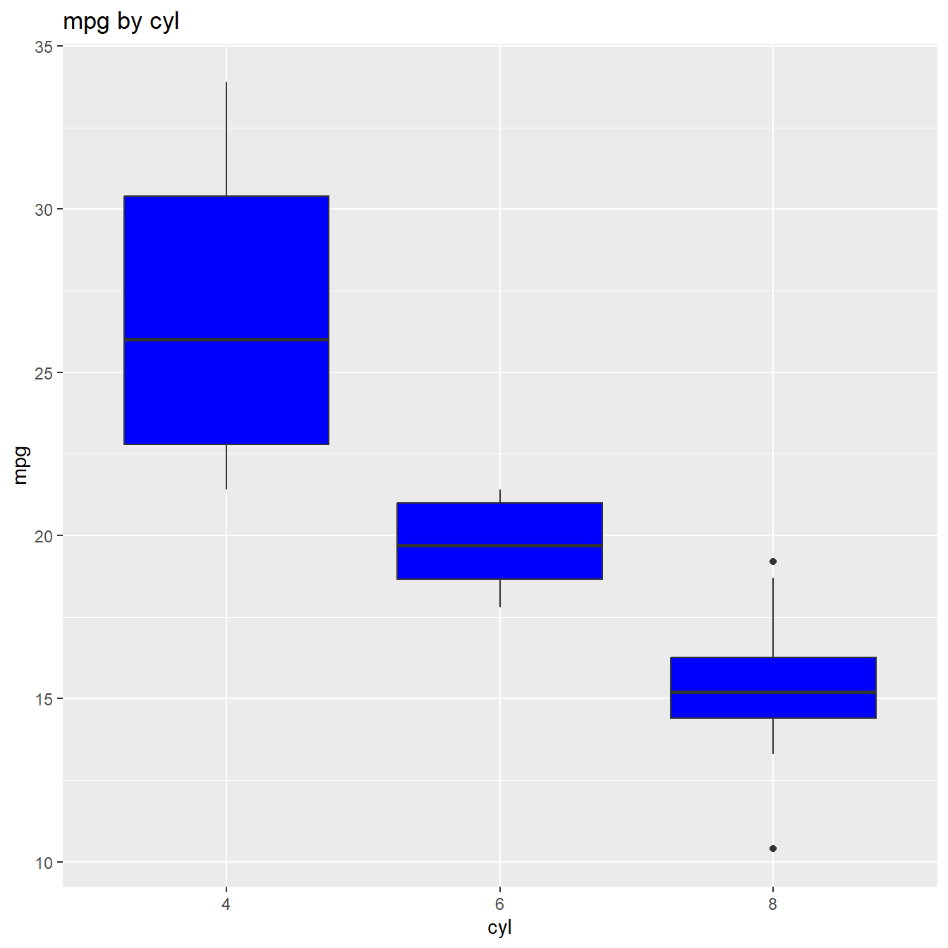
Multiple Variables
If you want grouped summary statistics for multiple variables in a data set, use ds_auto_group_summary().
ds_auto_group_summary(mtcarz, cyl, gear, mpg) by
-----------------------------------------------------------------------------------------
| Statistic/Levels| 4| 6| 8|
-----------------------------------------------------------------------------------------
| Obs| 11| 7| 14|
| Minimum| 21.4| 17.8| 10.4|
| Maximum| 33.9| 21.4| 19.2|
| Mean| 26.66| 19.74| 15.1|
| Median| 26| 19.7| 15.2|
| Mode| 22.8| 21| 10.4|
| Std. Deviation| 4.51| 1.45| 2.56|
| Variance| 20.34| 2.11| 6.55|
| Skewness| 0.35| -0.26| -0.46|
| Kurtosis| -1.43| -1.83| 0.33|
| Uncorrected SS| 8023.83| 2741.14| 3277.34|
| Corrected SS| 203.39| 12.68| 85.2|
| Coeff Variation| 16.91| 7.36| 16.95|
| Std. Error Mean| 1.36| 0.55| 0.68|
| Range| 12.5| 3.6| 8.8|
| Interquartile Range| 7.6| 2.35| 1.85|
-----------------------------------------------------------------------------------------
by
-----------------------------------------------------------------------------------------
| Statistic/Levels| 3| 4| 5|
-----------------------------------------------------------------------------------------
| Obs| 15| 12| 5|
| Minimum| 10.4| 17.8| 15|
| Maximum| 21.5| 33.9| 30.4|
| Mean| 16.11| 24.53| 21.38|
| Median| 15.5| 22.8| 19.7|
| Mode| 10.4| 21| 15|
| Std. Deviation| 3.37| 5.28| 6.66|
| Variance| 11.37| 27.84| 44.34|
| Skewness| -0.09| 0.7| 0.56|
| Kurtosis| -0.38| -0.77| -1.83|
| Uncorrected SS| 4050.52| 7528.9| 2462.89|
| Corrected SS| 159.15| 306.29| 177.37|
| Coeff Variation| 20.93| 21.51| 31.15|
| Std. Error Mean| 0.87| 1.52| 2.98|
| Range| 11.1| 16.1| 15.4|
| Interquartile Range| 3.9| 7.08| 10.2|
-----------------------------------------------------------------------------------------Multiple Variable Statistics
The ds_tidy_stats() function returns summary/descriptive statistics for variables in a data frame/tibble.
ds_tidy_stats(mtcarz, mpg, disp, hp)# A tibble: 3 × 16
vars min max mean t_mean median mode range variance stdev skew
<chr> <dbl> <dbl> <dbl> <dbl> <dbl> <dbl> <dbl> <dbl> <dbl> <dbl>
1 disp 71.1 472 231. 228 196. 276. 401. 15361. 124. 0.420
2 hp 52 335 147. 144. 123 110 283 4701. 68.6 0.799
3 mpg 10.4 33.9 20.1 20.0 19.2 10.4 23.5 36.3 6.03 0.672
# ℹ 5 more variables: kurtosis <dbl>, coeff_var <dbl>, q1 <dbl>, q3 <dbl>,
# iqrange <dbl>Measures
If you want to view the measure of location, variation, symmetry, percentiles and extreme observations as tibbles, use the below functions. All of them, except for ds_extreme_obs() will work with single or multiple variables. If you do not specify the variables, they will return the results for all the continuous variables in the data set.
Measures of Location
ds_measures_location(mtcarz) variable n missing mean trim_mean median mode
1 disp 32 0 230.72 228.00 196.30 275.80
2 drat 32 0 3.60 3.58 3.70 3.07
3 hp 32 0 146.69 143.57 123.00 110.00
4 mpg 32 0 20.09 19.95 19.20 10.40
5 qsec 32 0 17.85 17.79 17.71 17.02
6 wt 32 0 3.22 3.20 3.33 3.44Measures of Variation
ds_measures_variation(mtcarz) var n range iqr variance sd coeff_var std_error
1 disp 32 400.900 205.17500 1.536080e+04 123.9386938 53.71779 21.90947271
2 drat 32 2.170 0.84000 2.858814e-01 0.5346787 14.86638 0.09451874
3 hp 32 283.000 83.50000 4.700867e+03 68.5628685 46.74077 12.12031731
4 mpg 32 23.500 7.37500 3.632410e+01 6.0269481 29.99881 1.06542396
5 qsec 32 8.400 2.00750 3.193166e+00 1.7869432 10.01159 0.31588992
6 wt 32 3.911 1.02875 9.573790e-01 0.9784574 30.41285 0.17296847Measures of Symmetry
ds_measures_symmetry(mtcarz) var n skewness kurtosis
1 disp 32 0.4202331 -1.06752340
2 drat 32 0.2927802 -0.45043245
3 hp 32 0.7994067 0.27521159
4 mpg 32 0.6723771 -0.02200629
5 qsec 32 0.4063466 0.86493065
6 wt 32 0.4659161 0.41659467Percentiles
ds_percentiles(mtcarz) var n min per_1 per_5 per_10 q1 median q3 per_90
1 disp 32 71.100 72.52600 77.3500 80.6100 120.82500 196.300 326.00 396.0000
2 drat 32 2.760 2.76000 2.8535 3.0070 3.08000 3.695 3.92 4.2090
3 hp 32 52.000 55.10000 63.6500 66.0000 96.50000 123.000 180.00 243.5000
4 mpg 32 10.400 10.40000 11.9950 14.3400 15.42500 19.200 22.80 30.0900
5 qsec 32 14.500 14.53100 15.0455 15.5340 16.89250 17.710 18.90 19.9900
6 wt 32 1.513 1.54462 1.7360 1.9555 2.58125 3.325 3.61 4.0475
per_95 per_99 max
1 449.00000 468.28000 472.000
2 4.31450 4.77500 4.930
3 253.55000 312.99000 335.000
4 31.30000 33.43500 33.900
5 20.10450 22.06920 22.900
6 5.29275 5.39951 5.424Categorical Data
Cross Tabulation
The ds_cross_table() function creates two way tables of categorical variables.
ds_cross_table(mtcarz, cyl, gear) Cell Contents
|---------------|
| Frequency |
| Percent |
| Row Pct |
| Col Pct |
|---------------|
Total Observations: 32
----------------------------------------------------------------------------
| | gear |
----------------------------------------------------------------------------
| cyl | 3 | 4 | 5 | Row Total |
----------------------------------------------------------------------------
| 4 | 1 | 8 | 2 | 11 |
| | 0.031 | 0.25 | 0.062 | |
| | 0.09 | 0.73 | 0.18 | 0.34 |
| | 0.07 | 0.67 | 0.4 | |
----------------------------------------------------------------------------
| 6 | 2 | 4 | 1 | 7 |
| | 0.062 | 0.125 | 0.031 | |
| | 0.29 | 0.57 | 0.14 | 0.22 |
| | 0.13 | 0.33 | 0.2 | |
----------------------------------------------------------------------------
| 8 | 12 | 0 | 2 | 14 |
| | 0.375 | 0 | 0.062 | |
| | 0.86 | 0 | 0.14 | 0.44 |
| | 0.8 | 0 | 0.4 | |
----------------------------------------------------------------------------
| Column Total | 15 | 12 | 5 | 32 |
| | 0.468 | 0.375 | 0.155 | |
----------------------------------------------------------------------------If you want the above result as a tibble, use ds_twoway_table().
ds_twoway_table(mtcarz, cyl, gear)Joining with `by = join_by(cyl, gear, count)`# A tibble: 8 × 6
cyl gear count percent row_percent col_percent
<fct> <fct> <int> <dbl> <dbl> <dbl>
1 4 3 1 0.0312 0.0909 0.0667
2 4 4 8 0.25 0.727 0.667
3 4 5 2 0.0625 0.182 0.4
4 6 3 2 0.0625 0.286 0.133
5 6 4 4 0.125 0.571 0.333
6 6 5 1 0.0312 0.143 0.2
7 8 3 12 0.375 0.857 0.8
8 8 5 2 0.0625 0.143 0.4 A plot() method has been defined which will generate:
Grouped Bar Plots
k <- ds_cross_table(mtcarz, cyl, gear)
plot(k)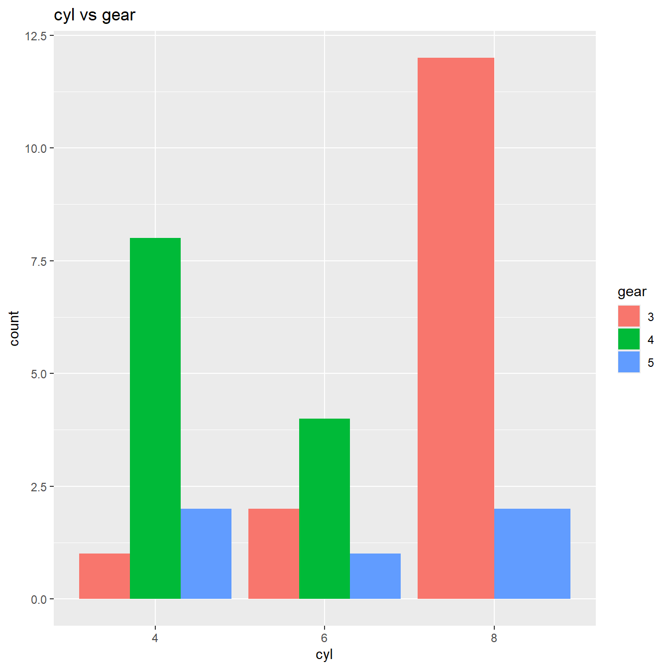
Stacked Bar Plots
k <- ds_cross_table(mtcarz, cyl, gear)
plot(k, stacked = TRUE)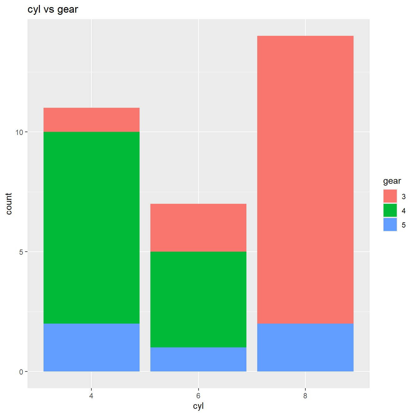
Proportional Bar Plots
k <- ds_cross_table(mtcarz, cyl, gear)
plot(k, proportional = TRUE)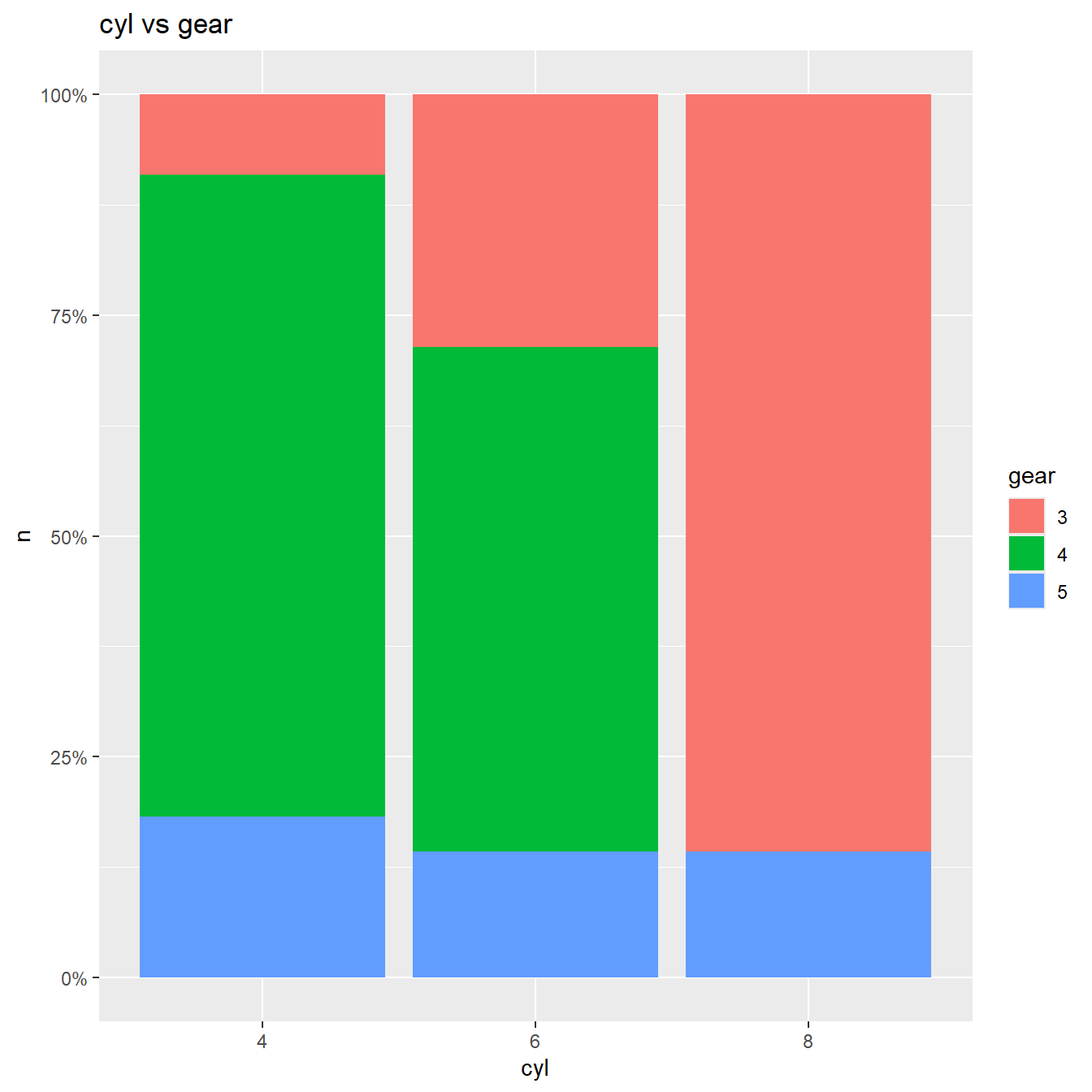
Frequency Table
The ds_freq_table() function creates frequency tables.
ds_freq_table(mtcarz, cyl) Variable: cyl
-----------------------------------------------------------------------
Levels Frequency Cum Frequency Percent Cum Percent
-----------------------------------------------------------------------
4 11 11 34.38 34.38
-----------------------------------------------------------------------
6 7 18 21.88 56.25
-----------------------------------------------------------------------
8 14 32 43.75 100
-----------------------------------------------------------------------
Total 32 - 100.00 -
-----------------------------------------------------------------------A plot() method has been defined which will create a bar plot.
k <- ds_freq_table(mtcarz, cyl)
plot(k)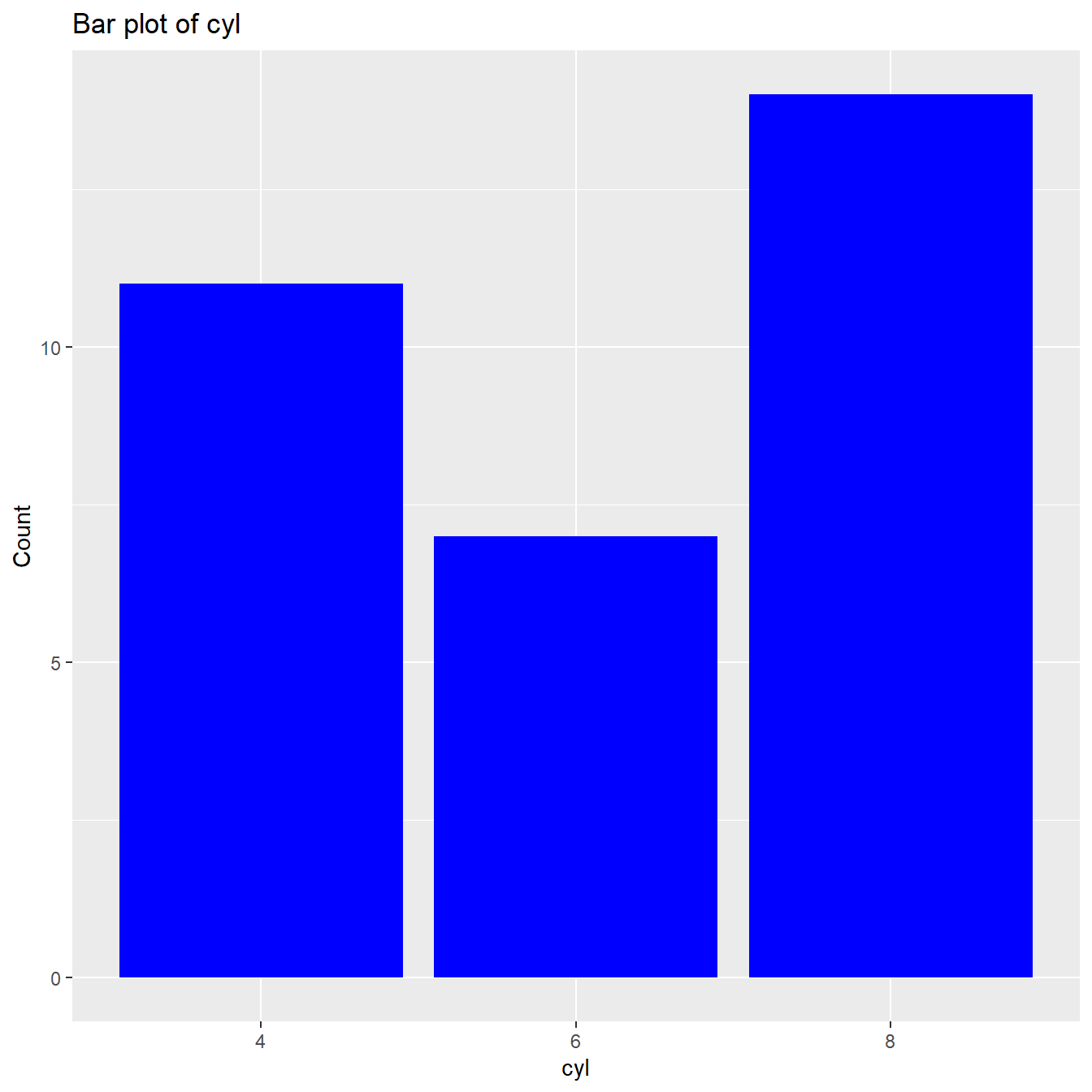
Multiple One Way Tables
The ds_auto_freq_table() function creates multiple one way tables by creating a frequency table for each categorical variable in a data set. You can also specify a subset of variables if you do not want all the variables in the data set to be used.
ds_auto_freq_table(mtcarz) Variable: cyl
-----------------------------------------------------------------------
Levels Frequency Cum Frequency Percent Cum Percent
-----------------------------------------------------------------------
4 11 11 34.38 34.38
-----------------------------------------------------------------------
6 7 18 21.88 56.25
-----------------------------------------------------------------------
8 14 32 43.75 100
-----------------------------------------------------------------------
Total 32 - 100.00 -
-----------------------------------------------------------------------
Variable: vs
-----------------------------------------------------------------------
Levels Frequency Cum Frequency Percent Cum Percent
-----------------------------------------------------------------------
0 18 18 56.25 56.25
-----------------------------------------------------------------------
1 14 32 43.75 100
-----------------------------------------------------------------------
Total 32 - 100.00 -
-----------------------------------------------------------------------
Variable: am
-----------------------------------------------------------------------
Levels Frequency Cum Frequency Percent Cum Percent
-----------------------------------------------------------------------
0 19 19 59.38 59.38
-----------------------------------------------------------------------
1 13 32 40.62 100
-----------------------------------------------------------------------
Total 32 - 100.00 -
-----------------------------------------------------------------------
Variable: gear
-----------------------------------------------------------------------
Levels Frequency Cum Frequency Percent Cum Percent
-----------------------------------------------------------------------
3 15 15 46.88 46.88
-----------------------------------------------------------------------
4 12 27 37.5 84.38
-----------------------------------------------------------------------
5 5 32 15.62 100
-----------------------------------------------------------------------
Total 32 - 100.00 -
-----------------------------------------------------------------------
Variable: carb
-----------------------------------------------------------------------
Levels Frequency Cum Frequency Percent Cum Percent
-----------------------------------------------------------------------
1 7 7 21.88 21.88
-----------------------------------------------------------------------
2 10 17 31.25 53.12
-----------------------------------------------------------------------
3 3 20 9.38 62.5
-----------------------------------------------------------------------
4 10 30 31.25 93.75
-----------------------------------------------------------------------
6 1 31 3.12 96.88
-----------------------------------------------------------------------
8 1 32 3.12 100
-----------------------------------------------------------------------
Total 32 - 100.00 -
-----------------------------------------------------------------------Multiple Two Way Tables
The ds_auto_cross_table() function creates multiple two way tables by creating a cross table for each unique pair of categorical variables in a data set. You can also specify a subset of variables if you do not want all the variables in the data set to be used.
ds_auto_cross_table(mtcarz, cyl, gear, am) Cell Contents
|---------------|
| Frequency |
| Percent |
| Row Pct |
| Col Pct |
|---------------|
Total Observations: 32
cyl vs gear
----------------------------------------------------------------------------
| | gear |
----------------------------------------------------------------------------
| cyl | 3 | 4 | 5 | Row Total |
----------------------------------------------------------------------------
| 4 | 1 | 8 | 2 | 11 |
| | 0.031 | 0.25 | 0.062 | |
| | 0.09 | 0.73 | 0.18 | 0.34 |
| | 0.07 | 0.67 | 0.4 | |
----------------------------------------------------------------------------
| 6 | 2 | 4 | 1 | 7 |
| | 0.062 | 0.125 | 0.031 | |
| | 0.29 | 0.57 | 0.14 | 0.22 |
| | 0.13 | 0.33 | 0.2 | |
----------------------------------------------------------------------------
| 8 | 12 | 0 | 2 | 14 |
| | 0.375 | 0 | 0.062 | |
| | 0.86 | 0 | 0.14 | 0.44 |
| | 0.8 | 0 | 0.4 | |
----------------------------------------------------------------------------
| Column Total | 15 | 12 | 5 | 32 |
| | 0.468 | 0.375 | 0.155 | |
----------------------------------------------------------------------------
cyl vs am
-------------------------------------------------------------
| | am |
-------------------------------------------------------------
| cyl | 0 | 1 | Row Total |
-------------------------------------------------------------
| 4 | 3 | 8 | 11 |
| | 0.094 | 0.25 | |
| | 0.27 | 0.73 | 0.34 |
| | 0.16 | 0.62 | |
-------------------------------------------------------------
| 6 | 4 | 3 | 7 |
| | 0.125 | 0.094 | |
| | 0.57 | 0.43 | 0.22 |
| | 0.21 | 0.23 | |
-------------------------------------------------------------
| 8 | 12 | 2 | 14 |
| | 0.375 | 0.062 | |
| | 0.86 | 0.14 | 0.44 |
| | 0.63 | 0.15 | |
-------------------------------------------------------------
| Column Total | 19 | 13 | 32 |
| | 0.594 | 0.406 | |
-------------------------------------------------------------
gear vs am
-------------------------------------------------------------
| | am |
-------------------------------------------------------------
| gear | 0 | 1 | Row Total |
-------------------------------------------------------------
| 3 | 15 | 0 | 15 |
| | 0.469 | 0 | |
| | 1 | 0 | 0.47 |
| | 0.79 | 0 | |
-------------------------------------------------------------
| 4 | 4 | 8 | 12 |
| | 0.125 | 0.25 | |
| | 0.33 | 0.67 | 0.38 |
| | 0.21 | 0.62 | |
-------------------------------------------------------------
| 5 | 0 | 5 | 5 |
| | 0 | 0.156 | |
| | 0 | 1 | 0.16 |
| | 0 | 0.38 | |
-------------------------------------------------------------
| Column Total | 19 | 13 | 32 |
| | 0.594 | 0.406 | |
-------------------------------------------------------------Learning More
The descriptr website includes comprehensive documentation on using the package, including the following articles that cover various aspects of using descriptr:
Continuous Data - for summarizing continuous data.
Categorical Data - for summarizing categorical data.
Visualization - for generating different types of plots.
Feedback
All feedback is welcome. Issues (bugs and feature requests) can be posted to github tracker. For help with code or other related questions, feel free to reach me hebbali.aravind@gmail.com.