# Install release version from CRAN
install.packages("olsrr")

# Install development version from GitHub
# install.packages("devtools")
devtools::install_github("rsquaredacademy/olsrr")Introducing olsrr
regression
Tools for linear regression.
I am pleased to announce the olsrr package, a set of tools for improved output from linear regression models, designed keeping in mind beginner/intermediate R users. The package includes:
- comprehensive regression output
- variable selection procedures
- heteroskedasticiy, collinearity diagnostics and measures of influence
- various plots and underlying data
If you know how to build models using lm(), you will find olsrr very useful. Most of the functions use an object of class lm as input. So you just need to build a model using lm() and then pass it onto the functions in olsrr. Once you have picked up enough knowledge of R, you can move on to more intuitive approach offered by tidymodels etc. as they offer more flexibility, which olsrr does not.
Installation
Shiny App
olsrr includes a shiny app which can be launched using
ols_launch_app()or try the live version here.
Read on to learn more about the features of olsrr, or see the olsrr website for detailed documentation on using the package.
Regression Output
model <- lm(mpg ~ disp + hp + wt + qsec, data = mtcars)
ols_regress(model)
Model Summary
---------------------------------------------------------------
R 0.914 RMSE 2.409
R-Squared 0.835 MSE 5.801
Adj. R-Squared 0.811 Coef. Var 13.051
Pred R-Squared 0.771 AIC 159.070
MAE 1.858 SBC 167.864
---------------------------------------------------------------
RMSE: Root Mean Square Error
MSE: Mean Square Error
MAE: Mean Absolute Error
AIC: Akaike Information Criteria
SBC: Schwarz Bayesian Criteria
ANOVA
--------------------------------------------------------------------
Sum of
Squares DF Mean Square F Sig.
--------------------------------------------------------------------
Regression 940.412 4 235.103 34.195 0.0000
Residual 185.635 27 6.875
Total 1126.047 31
--------------------------------------------------------------------
Parameter Estimates
----------------------------------------------------------------------------------------
model Beta Std. Error Std. Beta t Sig lower upper
----------------------------------------------------------------------------------------
(Intercept) 27.330 8.639 3.164 0.004 9.604 45.055
disp 0.003 0.011 0.055 0.248 0.806 -0.019 0.025
hp -0.019 0.016 -0.212 -1.196 0.242 -0.051 0.013
wt -4.609 1.266 -0.748 -3.641 0.001 -7.206 -2.012
qsec 0.544 0.466 0.161 1.166 0.254 -0.413 1.501
----------------------------------------------------------------------------------------In the presence of interaction terms in the model, the predictors are scaled and centered before computing the standardized betas. ols_regress() will detect interaction terms automatically but in case you have created a new variable instead of using the inline function, you can indicate the presence of interaction terms by setting iterm to TRUE.
Residual Diagnostics
olsrr offers tools for detecting violation of standard regression assumptions:
- Residual QQ plot
- Residual normality test
- Residual vs Fitted plot
- Residual histogram
ols_plot_resid_qq(model)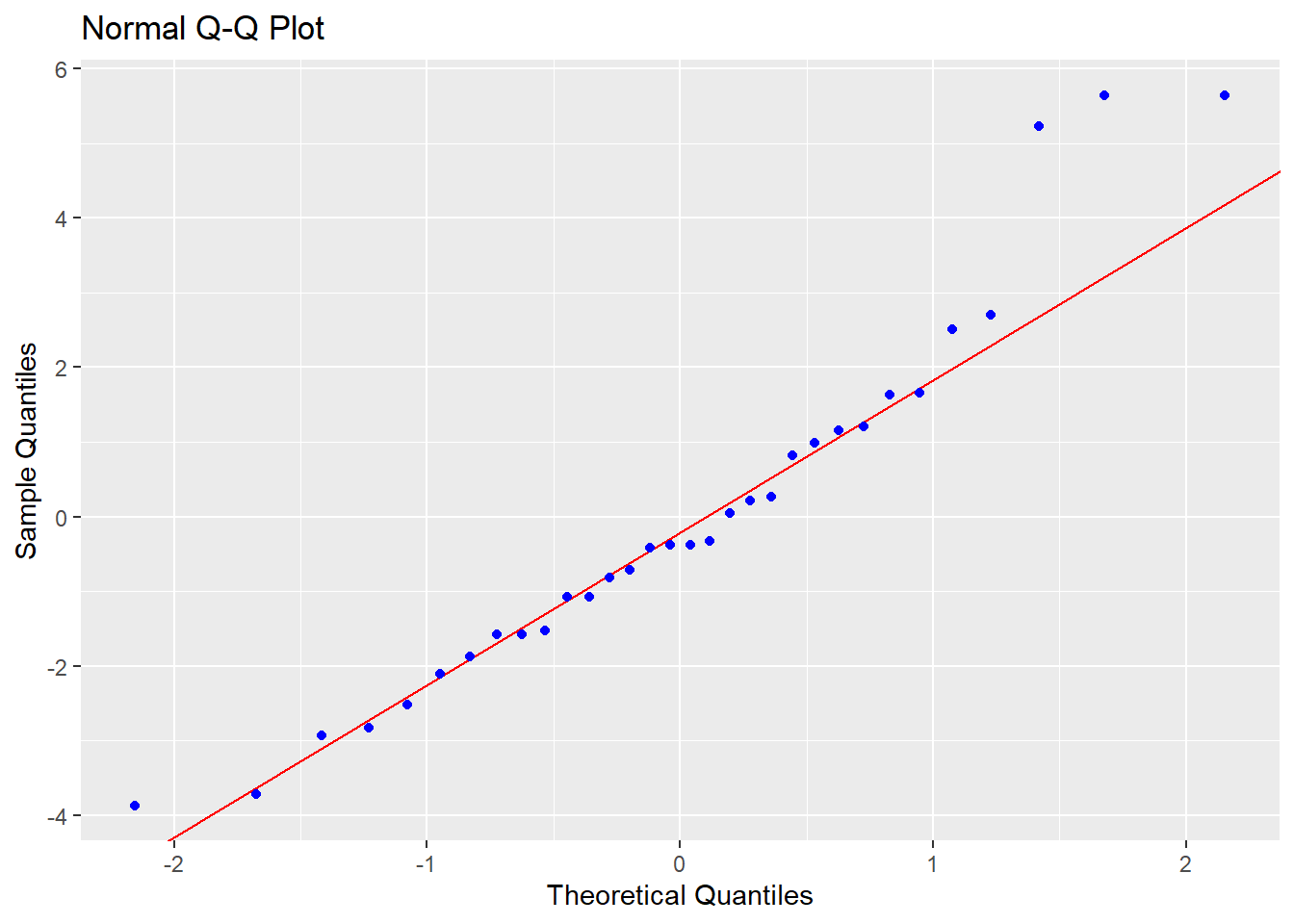
See Residual Diagnostics for more details.
Heteroskedasticity
olsrr provides the following 4 tests for detecting heteroscedasticity:
- Bartlett Test
- Breusch Pagan Test
- Score Test
- F Test
ols_test_breusch_pagan(model)
 Breusch Pagan Test for Heteroskedasticity
 -----------------------------------------
 Ho: the variance is constant
 Ha: the variance is not constant

             Data
 -------------------------------
 Response : mpg
 Variables: fitted values of mpg

        Test Summary
 ----------------------------
 DF            =    1
 Chi2          =    0.5884673
 Prob > Chi2   =    0.4430124
See Heteroskedasticity for more details.
Collinearity Diagnostics
VIF, Tolerance and condition indices to detect collinearity and plots for assessing mode fit and contributions of variables.
ols_coll_diag(model)Tolerance and Variance Inflation Factor
---------------------------------------
Variables Tolerance VIF
1 disp 0.1252279 7.985439
2 hp 0.1935450 5.166758
3 wt 0.1445726 6.916942
4 qsec 0.3191708 3.133119
Eigenvalue and Condition Index
------------------------------
Eigenvalue Condition Index intercept disp hp wt
1 4.721487187 1.000000 0.000123237 0.001132468 0.001413094 0.0005253393
2 0.216562203 4.669260 0.002617424 0.036811051 0.027751289 0.0002096014
3 0.050416837 9.677242 0.001656551 0.120881424 0.392366164 0.0377028008
4 0.010104757 21.616057 0.025805998 0.777260487 0.059594623 0.7017528428
5 0.001429017 57.480524 0.969796790 0.063914571 0.518874831 0.2598094157
qsec
1 0.0001277169
2 0.0046789491
3 0.0001952599
4 0.0024577686
5 0.9925403056See Collinearity Diagnostics for more details.
Measures of Influence
olsrr offers the following tools to detect influential observations:
- Cook’s D Bar Plot
- Cook’s D Chart
- DFBETAs Panel
- DFFITs Plot
- Studentized Residual Plot
- Standardized Residual Chart
- Studentized Residuals vs Leverage Plot
- Deleted Studentized Residual vs Fitted Values Plot
- Hadi Plot
- Potential Residual Plot
ols_plot_resid_lev(model)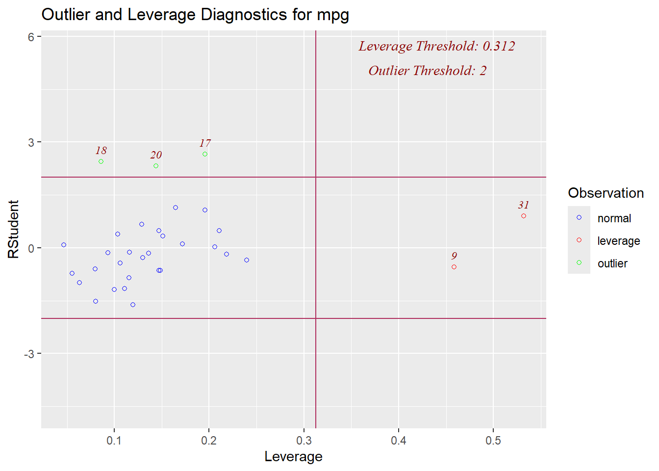
See Measures of Influence for more details.
Variable Selection
Different variable selection procedures such as all possible regression, best subset regression, stepwise regression, stepwise forward regression and stepwise backward regression.
model <- lm(y ~ ., data = stepdata)
ols_step_both_aic(model)
                                 Stepwise Summary
--------------------------------------------------------------------------------
Step    Variable         AIC          SBC          SBIC         R2       Adj. R2
--------------------------------------------------------------------------------
 0      Base Model    56988.482    57004.289       228.318    0.00000    0.00000
 1      x6 (+)        33473.297    33497.007    -23285.069    0.69145    0.69143
 2      x1 (+)        32931.758    32963.372    -23826.833    0.69972    0.69969
 3      x3 (+)        31912.722    31952.239    -24845.827    0.71466    0.71462
 4      x2 (+)        29304.296    29351.717    -27453.243    0.74958    0.74953
 5      x6 (-)        29302.317    29341.835    -27455.223    0.74958    0.74954
 6      x4 (+)        29300.814    29348.235    -27456.724    0.74962    0.74957
--------------------------------------------------------------------------------

Final Model Output
------------------

                          Model Summary
-----------------------------------------------------------------
R                       0.866       RMSE                   0.503
R-Squared               0.750       MSE                    0.253
Adj. R-Squared          0.750       Coef. Var           6430.859
Pred R-Squared          0.749       AIC                29300.814
MAE                     0.402       SBC                29348.235
-----------------------------------------------------------------
 RMSE: Root Mean Square Error
 MSE: Mean Square Error
 MAE: Mean Absolute Error
 AIC: Akaike Information Criteria
 SBC: Schwarz Bayesian Criteria

                                   ANOVA
---------------------------------------------------------------------------
                 Sum of
                Squares           DF    Mean Square        F          Sig.
---------------------------------------------------------------------------
Regression    15163.528            4       3790.882    14966.061    0.0000
Residual       5064.705        19995          0.253
Total         20228.233        19999
---------------------------------------------------------------------------

                                  Parameter Estimates
---------------------------------------------------------------------------------------
      model      Beta    Std. Error    Std. Beta      t        Sig      lower    upper
---------------------------------------------------------------------------------------
(Intercept)    -0.005         0.004                 -1.496    0.135    -0.012    0.002
         x1     0.255         0.003        0.362    84.140    0.000     0.249    0.261
         x3     0.253         0.003        0.356    82.604    0.000     0.247    0.259
         x2     0.249         0.003        0.346    80.544    0.000     0.243    0.255
         x4    -0.007         0.004       -0.007    -1.872    0.061    -0.014    0.000
---------------------------------------------------------------------------------------
See Variable Selection for more details.
Learning More
The olsrr website includes comprehensive documentation on using the package, including the following articles that cover various aspects of using olsrr:
Variable Selection - Different variable selection procedures such as all possible regression, best subset regression, stepwise regression, stepwise forward regression and stepwise backward regression.
Residual Diagnostics - Includes plots to examine residuals to validate OLS assumptions.
Heteroskedasticity - Tests for heteroskedasticity include bartlett test, breusch pagan test, score test and f test.
Collinearity Diagnostics - VIF, Tolerance and condition indices to detect collinearity and plots for assessing mode fit and contributions of variables.
Measures of Influence - Includes 10 different plots to detect and identify influential observations.
Feedback
olsrr has been on CRAN for more than an year while we were fixing bugs and making the API stable. All feedback is welcome. Issues (bugs and feature requests) can be posted to github tracker. For help with code or other related questions, feel free to reach me hebbali.aravind@gmail.com.